

Key takeaways
Use sensitivity analysis to answer a decision question.
Choose assumptions that could affect the actual decision and identify the evidence needed to reduce uncertainty instead of displaying an unexplained wide range.
Distinguish isolated stresses from coherent scenarios.
A one-variable test holds other inputs fixed; a scenario should model connected effects on earnings, operating funding and cash together.
Show equity effects as well as operating value.
Fixed debt can amplify percentage movements in equity, so a percentage change in enterprise value does not necessarily imply the same percentage change in share value.
Do not label grid extremes as a valuation conclusion.
Illustrative factors and corner outputs are diagnostic stresses, not market benchmarks, probability estimates or a statistically supported fair-value interval.
Reconcile interactions and avoid duplicate risk charges.
Multiplicative assumptions interact, and cash or working-capital movements can offset operating changes; explain each effect without charging twice for the same risk.
Ask which uncertainty could change the decision
A valuation sensitivity analysis shows how a result changes when a specified assumption changes. Its purpose is not to produce the widest possible range. It should identify the assumptions that matter, explain plausible alternatives and direct attention to evidence that could improve a decision. A spreadsheet with many coloured cells can still fail that test.
Start by identifying the decision: whether to accept a sale offer, investigate customer concentration, fund expansion or negotiate an ownership transfer. Then state the valuation date, subject, basis and method. A sensitivity in enterprise value is not automatically a sensitivity in the value of an owner's shares, and neither is necessarily a change in immediate sale proceeds.
Australian Government guidance describes different valuation methods and the underlying financial and business information required. The analysis must remain consistent with the selected method; a sensitivity table does not make an unsuitable method appropriate. Australian Government guidance on valuing a business
Separate a sensitivity from a scenario
A one-variable sensitivity changes one input while holding the others fixed. It is useful for seeing the mechanical effect of, for example, an alternative replacement salary. A scenario changes a connected group of assumptions to describe a coherent possible outcome. Losing a major customer may change revenue, staffing, margin and working-capital needs together.
Neither exercise is automatically a probability forecast. A downside case does not have a 25% likelihood because it occupies one of four columns. A minimum and maximum from a grid are not a statistical confidence interval. If probabilities are used, explain their evidence and whether the outcomes are mutually exclusive and sufficiently complete.
The ATO's market valuation guidance expects information relevant to the valuation date, rather than an answer reconstructed using hindsight. For a tax purpose, check that guidance directly; for another purpose, do not assume its requirements define the whole engagement. The useful discipline is to label what was known, what was foreseeable and what is hypothetical. ATO market valuation guidance
Fictional base case with explicit funding assumptions
All figures in this example are fictional Australian dollars. Wattle Maintenance Pty Ltd is a standalone business with no subsidiaries, preference shares or group non-controlling interests. The subject is all ordinary equity, not a particular minority parcel. No control premium or lack-of-control or marketability discount is modelled; an individual holding would need separate rights and basis analysis rather than automatic pro-rata fair value.
Assume normalised EBITDA of $600,000 and a supplied capitalisation factor of 4.0. Enterprise value is $600,000 × 4.0 = $2,400,000. These are teaching inputs, not evidence of Australian market multiples or an appropriate range for any real business. The factor would require independent support before use in an actual valuation.
Enterprise value includes normal operating assets, a required $80,000 cash float and normal non-cash working capital of $300,000. Total cash is $200,000, so only $120,000 surplus cash is added. Bank debt is $500,000 and equipment finance is $100,000. Actual eligible non-cash working capital is $280,000, leaving a $20,000 shortfall. There are no shareholder loans, lease liabilities, non-operating assets or other adjustments; premises rent is included in earnings.
All-share equity value is therefore $2,400,000 + $120,000 − $500,000 − $100,000 − $20,000 = $1,900,000. Other tax balances and contingent liabilities are assumed nil. Taxes on a sale, transaction costs, escrow and payment timing are excluded. Every subsequent result should show whether these funding assumptions remain unchanged.

Signed
A clear valuation conclusion starts with an agreed purpose, relevant evidence and disclosed assumptions. The report identifies the interest valued and explains the reasoning behind its conclusion.
Test earnings while holding the factor constant
First vary EBITDA to $540,000, $600,000 and $660,000 while keeping the factor at 4.0 and every equity-bridge adjustment fixed. Enterprise values are $2,160,000, $2,400,000 and $2,640,000. The fixed bridge adjustment totals negative $500,000, so corresponding all-share equity values are $1,660,000, $1,900,000 and $2,140,000.
A $60,000 EBITDA change therefore moves enterprise and equity value by $240,000 in this deliberately linear model. A 10% change in EBITDA moves base equity value by approximately 12.6%, not 10%, because debt and the other bridge items do not change. Show both the dollars and the denominator when discussing percentage movements.
This test isolates earnings uncertainty; it does not establish that earnings can change without affecting receivables, stock, staffing or cash. For a short diagnostic that simplification may be useful. For a business forecast, it may be inadequate. State it explicitly rather than letting readers infer a complete economic forecast from a multiplication exercise.
Test the capitalisation judgement separately
Now hold EBITDA at $600,000 and test factors of 3.5, 4.0 and 4.5. Enterprise values become $2,100,000, $2,400,000 and $2,700,000; equity values are $1,600,000, $1,900,000 and $2,200,000 after the unchanged negative $500,000 bridge. These factor changes are arbitrary teaching stresses, not market benchmarks or an evidence-supported valuation interval.
If the low earnings input and low factor are combined, enterprise value is $540,000 × 3.5 = $1,890,000 and equity value is $1,390,000. The combined high corner is $660,000 × 4.5 = $2,970,000 enterprise value and $2,470,000 equity value. Those corner outputs show mathematical exposure, not the endpoints of a concluded fair-value range.
Multiplicative inputs interact. In the high corner, the earnings increase alone contributes $240,000, the factor increase alone $300,000 and their interaction $30,000. Together they explain the $570,000 rise from base enterprise value. Summing only the first two effects would miss the interaction and fail to reconcile the model.
Build one coherent customer-loss scenario
Suppose a fictional customer loss removes $300,000 annual revenue but avoids $180,000 of genuinely variable costs. No fixed staff savings are assumed. EBITDA falls by $120,000 to $480,000. Holding the factor at 4.0 solely to isolate operating effects produces enterprise value of $1,920,000.
For this scenario, assume required non-cash working capital falls from $300,000 to $250,000. Actual eligible balances fall from $280,000 to $250,000 through collection and inventory conversion, releasing $30,000 into cash. Required operating cash remains $80,000; total cash rises from $200,000 to $230,000, leaving surplus cash of $150,000. Debt remains $600,000 and the working-capital shortfall disappears.
Scenario equity value is $1,920,000 + $150,000 − $600,000 = $1,470,000. The $430,000 decline from base equity reconciles to negative $480,000 operating value, positive $30,000 surplus cash and positive $20,000 removal of the shortfall. The result assumes the stated conversion of balances is achievable at the scenario measurement date, without losses, restructuring costs or additional tax effects. It is not a forecast of an instantaneous customer departure.
Avoid charging for the same risk twice
A lower earnings forecast and a lower capitalisation factor may both be justified, but identify the distinct reason for each. If earnings already remove a customer's contribution, a second blanket deduction for that same lost contribution may duplicate the effect. A separate increase in uncertainty about remaining customers would need its own evidence.
For discounted cash flow, distinguish operating cash-flow sensitivities from discount-rate and terminal-value sensitivities. Check consistency between nominal or real amounts, inflation, tax treatment and the relevant cash-flow recipient. Do not translate a change in an EBITDA factor into a discount-rate change without explaining the model relationship. Likewise, long-term growth cannot exceed what the business can fund simply because a cell allows it.
Use the output to prioritise evidence
Rank material assumptions by their effect on the decision, then identify the evidence needed: customer contracts, margin records, replacement-cost estimates, maintenance plans or working-capital reconciliations. A reverse sensitivity can ask what EBITDA would be required to reach a specified equity value, but that result is a hurdle to investigate, not proof the business can achieve it.
APESB distinguishes engagement types and their reporting and documentation requirements. IBV voluntarily aligns with APES 225 rather than being bound by it; the agreed scope must explain limitations on evidence and analysis. APESB guidance on valuation services
Preserve a labelled base model and a change log. A reviewer should be able to reproduce each result and see what did not change. That makes sensitivity analysis useful for decisions without mistaking model precision for certainty about value.
For the underlying approaches, see business valuation methods explained. Confirm the valuation purpose, intended users and information available before relying on a report.
Frequently asked questions
What does valuation sensitivity analysis show?
It shows the mechanical effect of changing specified assumptions while stating what remains fixed. It helps identify material uncertainties but does not remove the need for an evidenced valuation conclusion.
How is a scenario different from a sensitivity?
A sensitivity commonly changes one input. A scenario changes connected assumptions, such as revenue, variable costs and operating funding after a customer loss.
Are the example's factors of 3.5 to 4.5 Australian market multiples?
No. They are invented teaching stresses, not observed market evidence or a recommended range for a real business.
Why does a 10% EBITDA change move equity by about 12.6%?
At the fixed factor, EBITDA changes enterprise value by $240,000. Relative to base equity of $1,900,000, that is approximately 12.6%, because the funding bridge remains fixed.
Can the lowest and highest grid cells be called a fair-value range?
Not from the grid alone. The endpoints need support for their assumptions, combinations and applicable valuation basis; a mathematical envelope is not a concluded range.
What is an interaction effect?
When two multiplied inputs change, part of the result comes from their combined movement. The fictional high corner includes a $30,000 interaction beyond the separate earnings and factor effects.
Why does the customer-loss scenario release only $30,000 cash?
Actual working capital falls from $280,000 to $250,000. The required target falls by $50,000, but that is not itself a $50,000 cash receipt; the separate $20,000 shortfall disappears.
Should a customer loss also reduce the capitalisation factor?
Possibly, if there is a distinct supported change in risk. Explain that change rather than charging a second time for contribution already removed from earnings.
Do sensitivity tables assign probabilities to outcomes?
Not unless probabilities are separately justified. A downside column has no automatic likelihood, and a grid is not a confidence interval.
Can the analysis value an individual minority shareholding?
Not automatically. The fictional analysis concerns all ordinary equity; a particular holding requires assessment of its rights, restrictions and valuation basis before any parcel adjustment or allocation.
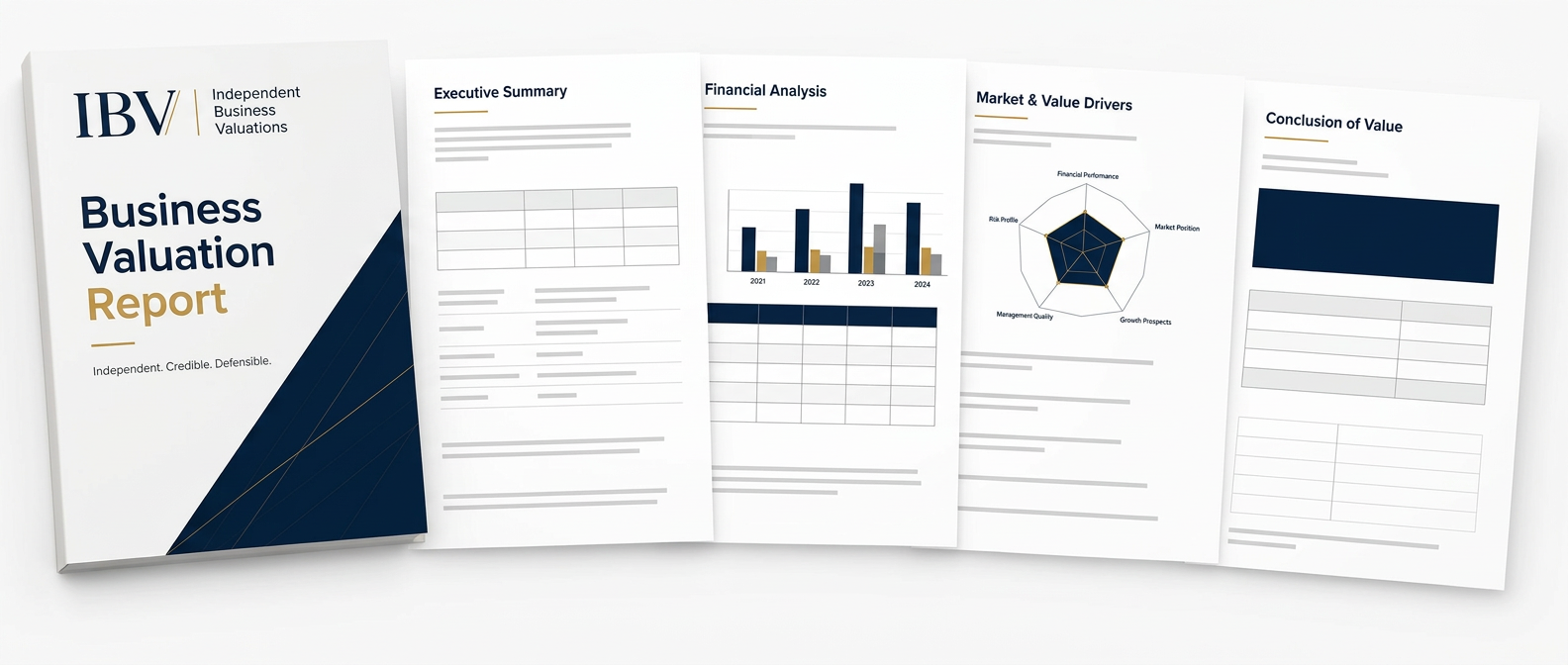
A clear, independent view of value — with the evidence behind it.
- Understand the conclusion — and what drives value.
- Gain an independent perspective. Move forward with confidence.
- Benchmark your business against industry performance.
- Identify strengths, risks and opportunities through SWOT analysis.
WHAT YOU GET IN A LIMITED SCOPE VALUATION REPORT
Inside your IBV™ report
Executive Summary
Conclusion of value · Method selected · Valuer qualifications
Detailed Report
Maintainable earnings · Cap rate / multiple · Premise of value
The Evidence Pack
SWOT analysis · Top Performers Report · RAVDA score
APES 225 voluntarily aligned. Report depth and supporting analysis follow your agreed package and engagement scope.
Free Valuation Call